Framing a data science problem is the process of converting a real-world challenge into a clear, solvable analytical task.
In data science, this step defines what problem to solve, what data is needed, and what type of analysis or model is appropriate.
Proper problem framing helps determine whether the task is descriptive, diagnostic, predictive, or prescriptive, and sets realistic expectations for outcomes.
Identifying the Type of Data Science Problem
One of the earliest decisions in framing a data science problem is determining the type of analytical problem you are solving.
Data science spans multiple categories—such as classification, prediction, clustering, optimization, anomaly detection, natural language processing, or recommendation systems—each requiring different techniques, evaluation metrics, and data preparation processes.
Understanding the problem type ensures that teams choose the right modeling strategy and avoid wasting time evaluating algorithms that are fundamentally unsuitable.
For Example, if the goal is to determine whether a customer is likely to churn (yes/no), this is a classification task. However, if the goal is to estimate how many days until the customer churns, it becomes a regression problem.
Project framing also depends heavily on whether the task is supervised, unsupervised, or semi-supervised. Supervised learning is used when historical outputs (labels) are available, such as predicting loan defaults.
Unsupervised learning is used when the goal is to uncover hidden patterns without predefined labels, such as grouping customers into segments. Semi-supervised learning bridges the gap when some labels exist but are not sufficient.
Another important consideration is whether the problem requires real-time processing or batch analysis.
Fraud detection, for example, demands immediate predictions, while monthly sales forecasting can be processed in scheduled batches. The nature of the problem directly impacts the architecture and computational resources required.
Properly identifying the problem type ensures that data scientists structure the entire workflow—from feature engineering to model deployment with clarity and precision.
Determining Target Variables and Outputs
Once the problem type is identified, the next step is to define the target variable (what the model aims to predict or discover) and the expected output format. This step links the business goal to the predictive or analytical task in a concrete way.
A clearly defined target variable ensures the model has a measurable, relevant outcome aligned with the objective.
For example, if a business wants to reduce customer churn, the target variable could be:
1. A binary label (“churn” or “not churn”)
2. A probability score (likelihood of churn)
3. A time-to-churn estimate
Each option drastically changes data preparation, modeling strategy, and intervention planning.
The output type also matters. A recommendation engine may output:
1. A ranked list of products
2. A similarity score between items
3. Personalized recommendations for each user segment
Meanwhile, an anomaly detection model may output:
1. A binary anomaly flag
2. An anomaly severity score
3. A list of suspicious events
The choice of output determines which features must be engineered and what evaluation metrics should be used.
For instance, predicting churn probability requires logistic regression metrics like AUC and log-loss, while predicting sales amounts requires regression metrics such as MAE or RMSE.
Clearly defining the output also helps stakeholders understand what the model will deliver. Without this clarity, business teams may expect insights or predictions the model was never designed to produce.
Ultimately, defining target variables and outputs ensures that the model and business expectations remain aligned throughout the project lifecycle.
Selecting Appropriate Analytical Approaches
After defining the target variable, teams must choose the analytical approach that best suits the problem.
Analytical approaches include descriptive analytics, statistical modeling, predictive machine learning, prescriptive analytics, simulation, optimization, or deep learning–based approaches.
This selection is not just about choosing an algorithm; it’s about selecting a methodological direction.
For example, if the goal is to forecast demand, statistical time-series models like ARIMA or exponential smoothing may suffice.
But if the problem requires capturing long-term dependencies or seasonality in complex patterns, advanced models such as LSTM neural networks may be more appropriate.
Similarly, for classification tasks, simple models like decision trees or logistic regression may work well if interpretability is crucial.
In contrast, random forests, gradient boosting (XGBoost, LightGBM), or neural networks may be selected when accuracy is the top priority.
Another decision involves choosing between rule-based approaches and machine-learning models. In situations where the domain is heavily regulated (e.g., banking), rule-based systems may be more appropriate due to transparency requirements.
Selecting the right analytical approach also involves aligning with available data. For example, deep learning models require large datasets, whereas traditional machine-learning methods perform well even with moderate data sizes.
This step ensures that the model is not only technically sound but also appropriate for the business context, available resources, and deployment requirements.
Understanding Constraints and Success Criteria
Effective problem framing requires understanding the constraints that limit the solution, as well as the success criteria that define when the project has achieved its goals.
Constraints
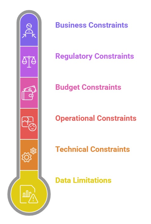
1. Data limitations: missing fields, poor quality, small sample sizes
2. Technical constraints: lack of infrastructure, slow systems, legacy databases
3. Operational constraints: deployment restrictions, integration challenges
4. Budget or time constraints: urgent timelines, limited engineering support
5. Regulatory constraints: data privacy laws, compliance issues
6. Business constraints: resistance to change, limited stakeholder engagement
Clearly identifying constraints during problem framing helps teams avoid unrealistic expectations and design solutions that are implementable within real-world limitations.
Success criteria define what “good” looks like for the project. This could be:
1. Achieving 80% churn prediction accuracy
2. Reducing manufacturing downtime by 15%
3. Increasing marketing ROI by 10%
4. Achieving model inference under 200 milliseconds
5. Delivering reports that enable weekly decision-making
Success criteria must be measurable, achievable, and agreed upon by all stakeholders.
Without shared success criteria, stakeholders may judge the final model inconsistently, leading to dissatisfaction or rejection of the solution.
Understanding constraints and success criteria ensures that the project remains practical, measurable, and aligned with the needs of the organization.
Mapping the Problem to Data Requirements
Mapping the Problem to Data Requirements is a crucial step in analytics and decision-making.
It focuses on clearly translating a business problem into specific data needs, ensuring the right data is collected, analyzed, and used to generate actionable insights.
Data Sources
Data Sources are the origins from which data is collected for analysis in the data science process.
They include internal systems, external platforms, and public datasets that provide the raw information needed to generate insights and build models.
Internal Data
1. CRM Systems
Customer Relationship Management systems store detailed information about customers, including their demographics, communication history, purchase patterns, and support interactions.
This data is extremely valuable because it helps businesses understand who their customers are, what they prefer, and how they behave across different touchpoints.
In data science projects, CRM data can be used to segment customers, predict churn, personalize marketing campaigns, or measure lifetime value.
Since the data originates directly from business activities, it is typically reliable, consistent, and rich in context.
2. Transaction Logs
Transaction logs capture every sale, purchase, refund, and financial interaction that occurs within a business.
These logs show the real-time flow of revenue and customer activity, making them vital for tasks like demand forecasting, sales prediction, fraud detection, and customer behavior analysis.
Because they include timestamps, product details, and payment methods, transaction logs help data scientists study how user actions change over time and which patterns indicate long-term loyalty or the risk of losing a customer.
3. Website Analytics
Website analytics include metrics such as page views, click paths, bounce rates, user sessions, and traffic sources.
This data reveals how visitors navigate a website, which pages they spend the most time on, and where they leave the site.
Data scientists use this information to improve user experience, identify pain points, optimize landing pages, and increase conversions.
Tools like Google Analytics provide structured insights into user behavior, making website data a powerful source for product optimization and marketing decisions.
4. Operational Data
Operational data comes from internal business processes such as supply chain movements, warehouse operations, employee activities, and service delivery workflows.
This type of data helps organizations understand how efficiently they function behind the scenes.
Data scientists use operational data to identify bottlenecks, improve productivity, measure performance, and reduce costs.
For example, analyzing warehouse activity logs can uncover delays, inventory inaccuracies, or inefficiencies in order fulfillment.
External Data
1. Market Data
Market data provides insights into industry trends, competitor pricing, consumer demand, and economic movements.
It is essential for benchmarking a company’s performance and positioning its products competitively.
Data scientists use market data to forecast demand shifts, adjust pricing strategies, design competitive marketing campaigns, and understand external influences that may affect business outcomes.
Because market conditions change rapidly, external market data helps organizations remain agile and informed.
2. Social Media Signals
Social media platforms provide massive volumes of real-time data such as mentions, comments, hashtags, shares, and sentiment reactions.
This data helps data scientists understand how people feel about a brand, product, or event.
By analyzing trends and patterns in online behavior, companies can detect emerging issues, measure the impact of marketing campaigns, or even predict viral trends.
Social media signals are especially critical for sentiment analysis, reputation management, and audience targeting.
3. Public Datasets
Governments, research institutes, and open-data platforms release large datasets covering topics like population statistics, environmental factors, transportation, healthcare, and education.
These free datasets help enrich internal project data or serve as the foundation for academic and exploratory projects.
In data science, public datasets are often used for model training, benchmarking, or gaining insights into broader societal patterns. They are also a great starting point for beginners learning to work with real-world data.
4. Vendor-Provided Data
Some organizations purchase specialized datasets from vendors to get insights they cannot obtain internally.
This might include demographic profiles, credit scoring information, geolocation data, or industry-specific intelligence.
Vendor data is typically high quality because it is curated by professionals, and it can significantly enhance predictive models when combined with internal data.
Although it comes at a cost, it often provides competitive advantages in analytics-driven decision-making.
Data Structure
Data structures classify information based on organization and format, influencing how it is stored, accessed, and analyzed.
Understanding structured, semi-structured, and unstructured data is essential for effective data processing and analytics.
1. Structured Data (Tables)
Structured data is well-organized in rows and columns, similar to an Excel spreadsheet or SQL database table.
Each row represents an entity (such as a customer), and each column represents an attribute (like age or purchase amount).
Because of its organization, structured data is easy to search, filter, visualize, and analyze.
Data scientists prefer structured data because most machine learning algorithms work naturally with it. Cleaning and preprocessing structured data is often simpler compared to other formats.
2. Semi-Structured Data (JSON, XML)
Semi-structured data does not fit perfectly into rows and columns, but it still contains labels and hierarchical organization.
Examples include API responses, server logs, messages, and configuration files. Although it is more flexible than structured data, it requires special parsing techniques to extract useful information.
Data scientists often convert semi-structured data into structured form before analysis. Semi-structured data is common in web applications and modern software systems, making it an essential skill for beginners to learn.
3. Unstructured Data (Text, Images, Audio, Video)
Unstructured data has no predefined format, making it harder to analyze directly.
This category includes emails, chat messages, customer reviews, social media posts, photos, voice recordings, and videos.
Because unstructured data captures natural human expression,
it is extremely valuable for advanced data science tasks like Natural Language Processing (NLP), image classification, speech recognition, and recommendation systems.
Processing unstructured data often requires specialized algorithms and techniques.
Data Coverage and Time Windows
Data coverage and time windows define the span and recency of data used for analysis, directly affecting model insights and accuracy.
Proper selection of historical and recent data ensures predictive models capture relevant patterns while avoiding outdated or incomplete information.
1. 12 Months of Transaction History
Having at least a year of transaction data helps data scientists identify long-term patterns such as seasonal trends, repeat purchase cycles, and the impact of promotions.
For example, some stores experience predictable sales increases during festivals or holidays each year.
Without sufficient historical data, models may fail to recognize these recurring patterns.
A 12-month window ensures that the model captures both short-term fluctuations and annual cycles.
2. 90-Day Activity Windows
Shorter windows such as 30-day or 90-day activity periods help data scientists understand recent customer behavior, which is highly relevant for predictive tasks like churn analysis.
Customers who have not logged in, purchased, or interacted within the last 90 days may be at higher risk of leaving.
These windows offer a snapshot of recency, making them ideal for models that rely on up-to-date behavioral trends rather than older historical behavior.
3. Customer Service Interaction Logs
These logs track how often a customer reaches out, what issues they face, and how their concerns were resolved.
Frequent complaints or unresolved issues may indicate dissatisfaction and can strongly predict churn.
Analyzing these logs helps data scientists uncover hidden patterns such as peak complaint times, common issues, and overall customer sentiment.
This data is useful for improving service quality and building customer satisfaction models.
4. Impact on Model Accuracy
The quantity and timeframe of data used directly influence the quality of machine learning predictions.
Short time windows may result in incomplete patterns, while excessively long windows might include outdated behavior no longer relevant.
Choosing the right time coverage ensures a balance between historical depth and current relevance, ultimately improving model reliability and accuracy.
Feature Engineering Needs
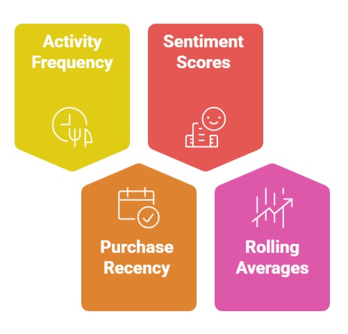
1. Customer Activity Frequency
Frequency measures how often a customer performs certain actions—visiting a website, purchasing a product, or contacting support.
High activity frequency often correlates with strong engagement and loyalty.
In predictive analytics, frequency features help identify active vs. inactive users and distinguish between high-value customers and occasional buyers.
These features are powerful indicators of future outcomes, such as purchase likelihood or service usage.
2. Purchase Recency
Recency refers to how recently a customer performed an action, usually a purchase. It is one of the strongest predictors of future behavior.
Customers who bought something recently are much more likely to buy again compared to customers who have been inactive for long periods.
Recency features help models understand customer lifecycle phases, making them essential for churn prediction, retention campaigns, and targeted marketing.
3. Sentiment Scores from Text
Sentiment analysis uses Natural Language Processing (NLP) to detect emotions expressed in text—positive, negative, or neutral.
Customer reviews, feedback forms, emails, and chat messages contain rich emotional signals that reveal satisfaction levels.
Converting raw text into sentiment scores helps data scientists quantify emotions and use them as features in models.
Sentiment features are critical for customer satisfaction analysis, brand monitoring, and complaint prediction.
4. Rolling Averages & Trend Features
Rolling averages smooth out short-term fluctuations by calculating the average of data points over a specific time window, such as 7 days or 30 days.
Trend features show whether a metric is increasing, decreasing, or stable over time.
These features are particularly important in time-series forecasting because they reveal underlying patterns and help models understand momentum.
Without these features, raw time-series data can be too noisy to produce accurate predictions.

Class Sessions
Sales Campaign

We have a sales campaign on our promoted courses and products. You can purchase 1 products at a discounted price up to 15% discount.