Forward and Reverse Diffusion Processes with Noise Scheduling are key concepts in generative modeling, particularly in diffusion-based models. In the forward diffusion process, data is gradually corrupted by adding noise over multiple steps until it becomes nearly random. This allows the model to learn how data transforms under noise.
The reverse diffusion process is the generative phase, where the model learns to denoise step by step, reconstructing data from pure noise back to a realistic sample.
Noise scheduling controls how noise is added during the forward process, which directly affects the quality and stability of the reverse generation. Choosing an appropriate noise schedule is crucial for efficient training and high-quality outputs.
Forward Diffusion Process
The forward diffusion process forms the foundation of diffusion models by simulating a gradual deterioration of data into pure noise.
Think of it as a controlled "noising" pipeline that transforms a crisp image into random static over many steps—mimicking natural entropy but in a mathematically structured way.
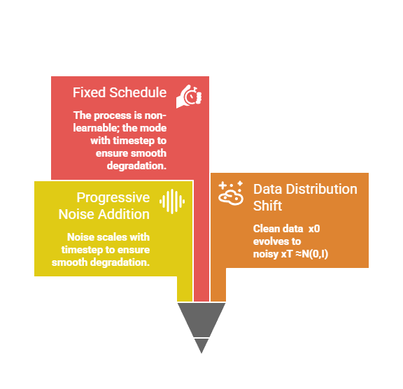
This process is deterministic and predefined, making it easy to replicate during training.
How Forward Diffusion Works
In the forward pass, we start with real data samples, like images from a dataset, and iteratively add small amounts of Gaussian noise. Each step corrupts the data a bit more, until it becomes indistinguishable from random noise.
This creates a Markov chain—a sequence where each state depends only on the previous one—spanning hundreds of timesteps, typically denoted as T (e.g., T=1000).
Key Characteristics
Here's a simplified Python snippet using NumPy to illustrate a single forward step (adaptable to PyTorch for real models)
import numpy as np


def forward_diffusion_step(x, t, beta_t):

    """Add noise to data x at timestep t using variance schedule beta_t."""

    alpha_t = 1 - beta_t

    noise = np.random.normal(0, np.sqrt(beta_t), x.shape)

    x_t = np.sqrt(alpha_t) * x + noise

    return x_t


# Example: x is a 1D image patch, beta_t from schedule

x_0 = np.array([0.5, 0.7, 0.2])  # Clean data

beta_1 = 0.0001  # Small noise variance at t=1

x_1 = forward_diffusion_step(x_0, 1, beta_1)
Role of Noise Schedules in Forward Process
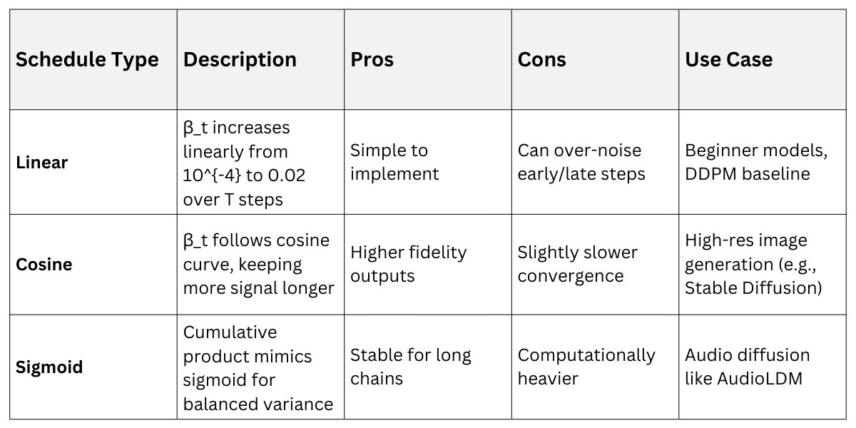
Noise scheduling controls how much noise is added at each timestep, preventing abrupt changes that could destabilize training. Linear schedules start small and increase steadily, while cosine schedules (introduced in Improved DDPM, 2021) curve more gently for better sample quality.
Practical Tip: In Hugging Face Diffusers library, switch schedules via scheduler = DDPMScheduler.from_pretrained("CompVis/stable-diffusion-v1-4", beta_schedule="cosine") for immediate quality boosts.
This scheduling ensures the forward process marks data with timestep embeddings, which the reverse process later uses to denoise intelligently.
Reverse Diffusion Process
The reverse diffusion process is where the magic happens: a neural network learns to undo the forward noise addition, step by step.
Imagine rewinding a video of sandcastles dissolving in the tide—the model predicts and subtracts noise to rebuild the original structure. Trained via score matching or variational bounds, it approximates the true posterior distribution at each step.
Training the Reverse Process
During training, the model (often a U-Net) takes noisy data xt and timestep t as input, predicting the noise added at that step. Loss is mean squared error between predicted and actual noise, enabling end-to-end learning without explicit likelihood computation.
The Process Unfolds in these Numbered Steps
1. Sample noisy input: Draw xt from forward process given real x0
2. Embed timestep: Convert t to sinusoidal embeddings (like in Transformers) for the model.
3. Predict noise: U-Net outputs ϵθ (xt ,t).
4. Compute loss: L= ∥ϵ−ϵθ (xt ,t)∥2
5. Update weights: Backpropagate via Adam optimizer.
Example from PyTorch (Hugging Face style)
from diffusers import DDPMScheduler, UNet2DModel

import torch


scheduler = DDPMScheduler(num_train_timesteps=1000)

model = UNet2DModel.from_pretrained("runwayml/stable-diffusion-v1-5", subfolder="unet")

noise = torch.randn((1, 4, 64, 64))  # Predicted noise target

timestep = torch.tensor([500])

noisy_latents = torch.randn((1, 4, 64, 64))

pred_noise = model(noisy_latents, timestep).sample

loss = torch.nn.functional.mse_loss(pred_noise, noise)
Inference: At test time, start from pure noise xT and iteratively denoise using the trained model—no ground truth needed. Sampling takes T steps but can be accelerated with DDIM or PLMS samplers.
Benefits
.png)
In Stable Diffusion, text prompts guide the reverse process, making it ideal for your course's prompt design focus.
Noise Scheduling in Practice
Noise scheduling bridges forward and reverse processes, dictating the "pace" of noising and denoising. Poor schedules lead to blurry outputs or training divergence; optimal ones preserve fine details.
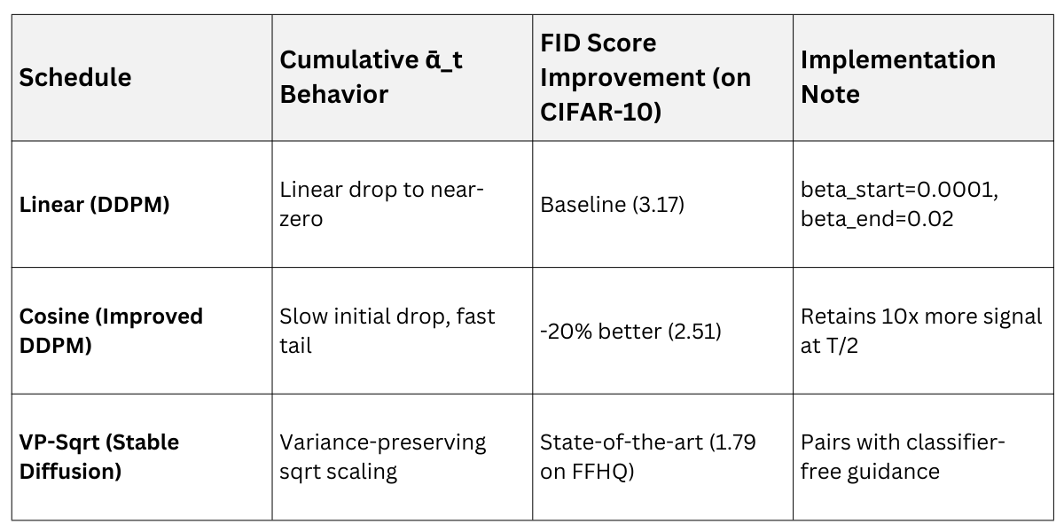
Industry standards from OpenAI and Stability AI favor cosine or VP (variance preserving) schedules for production models.
Comparing Popular Schedules
Advanced schedules adapt dynamically
Best Practices for Custom Schedules
When building your own diffusion model: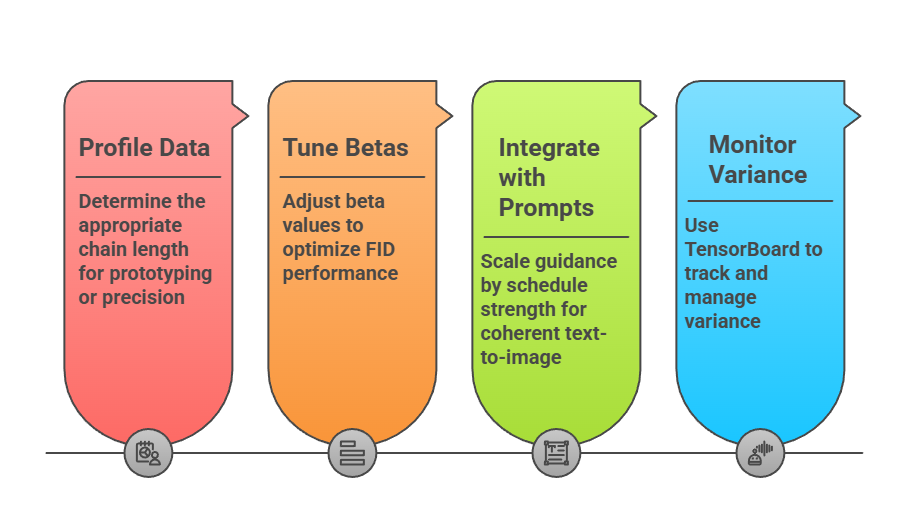
Real-world example: In healthcare data augmentation, use gentle cosine schedules to generate subtle variations of MRI scans without losing anatomical fidelity.
Integrating Diffusion in Generative Architectures
Diffusion processes shine in hybrid architectures, combining with VAEs (as in Stable Diffusion) for latent space efficiency. They handle prompt design elegantly—text encoders inject conditions into U-Net attention layers during reverse steps.
Practical project idea: Fine-tune Diffusers on your dataset with custom noise schedules to generate web UI mockups from prompts like "minimalist Delhi metro dashboard."
Class Sessions
Sales Campaign

We have a sales campaign on our promoted courses and products. You can purchase 1 products at a discounted price up to 15% discount.